感谢支持!您的打赏是我继续创作的动力!


Buffon 投针的计算机模拟
平面上画有间隔为 $d(d>0)$ 的等距平行线,向平面任意投掷一枚长为 $l(l< d)$ 的针。设 $x$ 为针的中点到最近平行线的垂直距离,$\varphi$ 为针与最近平行线所形成的夹角,于是样本空间 $\mit\Omega$ 就为
\[{\mathit\Omega}=\left\{(x,\varphi)\mid 0\leqslant x\leqslant\frac{d}{2},0\leqslant\varphi\leqslant\pi\right\}\]易知针与平行线相交的充分必要条件是:
\[\begin{equation} x\leqslant\frac{l}{2}\sin{\varphi} \end{equation}\]记事件 $A$ 为针与任一平行线相交,由几何概型可知
\[\begin{equation}\label{eq:Buffon} P(A)=\frac{S_A}{S_{\mathit\Omega}}=\frac{\displaystyle\int_{0}^{\pi}\frac{l}{2}\sin{\varphi}}{\frac{d}{2}\pi}=\frac{2l}{d\pi} \ (l<d) \end{equation}\]当实验次数 $N$ 足够大时,$P(A)\to\frac{n}{N}(N\to\infty)$,于是带入\eqref{eq:Buffon}式中,可解得
\[\begin{equation} \pi\approx\frac{2lN}{dn} \ (l<d) \end{equation}\]其中 $n$ 为针与任一平行线相交的次数。
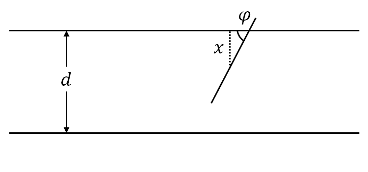
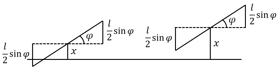
图 1: 比丰投针
我们用 R 语言来模拟 Buffon 投针的整个过程:
1
2
3
4
5
6
7
8
9
10
11
12
13
14
15
16
17
buffon <- function(toss_nums, needle_lengths, line_spacing) {
  if (needle_lengths >= line_spacing) {
  stop("Error: needle_lengths should be less than line_spacing!")
  }

  angle <- runif(n=toss_nums, 0, pi / 2)  # 针与平行线的角度
  dist_to_line <- runif(n=toss_nums, 0, line_spacing / 2)  # 针的中点到平行线的距离

  # 计算针的半径投影到平行线方向的长度
  projection_lengths <- needle_lengths / 2 * sin(angle)

  # 判断针是否与平行线相交
  hits <- sum(dist_to_line <= projection_lengths)

  pi_estimate <- (2 * needle_lengths * toss_nums) / (hits * line_spacing)
  return(pi_estimate)
}
- toss_nums:为 buffon 投针实验的投掷次数;
- needle_lenths:为实验所用的针的长度(cm);
- line_spacing:为实验两平行线间的距离(cm)。
当设置toss_nums=100000、needle_lengths=1、line_spacing=2时,则会输出
1
2
> buffon(100000, 1, 2)
[1] 3.15338
接下来对 Buffon 投针实验进行误差分析:
1
2
3
4
5
6
7
8
9
10
11
12
errors <- numeric(10000)
for (i in 1:10000) {
  error <- pi - buffon(10000, 1, 2)
  errors[i] <- error
}

hist(errors, probability = TRUE, main = "Buffon 投针误差直方图")

se <- sqrt(var(errors) / length(errors))
conf_upper <- mean(errors) + 1.96 * se
conf_lower <- mean(errors) - 1.96 * se
cat("置信区间:", c(conf_lower, conf_upper))
由结果可见,$\pi-\hat{\pi}$ 服从均值为 0 的正态分布。用 Python 来模拟的示例如下:
1
2
3
4
5
6
7
8
9
10
11
12
13
14
15
16
17
18
19
20
21
22
23
24
25
26
27
28
29
30
31
32
33
34
35
import numpy as np
import seaborn as sns
import matplotlib.pyplot as plt

def buffon(toss_nums, needle_lengths, line_spacing):
  if needle_lengths >= line_spacing:
  raise ValueError("Error: needle_lengths should be less than line_spacing!")

  dist_to_line = np.random.uniform(0, line_spacing / 2, size=toss_nums)  # 针的中点到平行线的距离
  angle = np.random.uniform(0, np.pi / 2, size=toss_nums)  # 针与平行线的角度

  # 计算针的半径投影到平行线的长度
  projection_lengths = needle_lengths / 2 * np.sin(angle)

  # 判断针是否与平行线相交
  hits = (dist_to_line <= projection_lengths).sum()

  pi_estimate = (2 * needle_lengths * toss_nums) / (hits * line_spacing)
  return pi_estimate

# 误差分析
errors = []
for i in range(10000):
  error = np.pi - buffon(10000, 1, 2)
  errors.append(error)

sns.histplot(errors, stat="density", bins="sturges", kde=True)
plt.xlabel("errors")
plt.title("Buffon 投针误差直方图")

# 95% 置信区间
se = np.sqrt(np.var(errors) / len(errors))
conf_upper = np.mean(errors) + 1.96 * se
conf_lower = np.mean(errors) - 1.96 * se
print(f"置信区间:({conf_lower}, {conf_upper})")
三门问题的计算机模拟
回顾一下三门问题的背景:你站在三个封闭的门前,其中一个门后有奖品,当然奖品在哪一个门后是完全随机的。当你选定一个门以后,主持人打开其余两扇门中的一扇空门,显示门后没有奖品。此时你可以有两种选择,保持原来的选择或者改选另一扇没有被打开的门。
当你作出最后选择以后,如果打开的门后有奖品,这个奖品就归你。现在有三种策略:
- 坚持原来的选择;
- 改选另一扇没有被打开的门。
我们已经知道若采取第 1 种策略,那么赢得奖品的概率为 $\frac{1}{3}$;若采取第 2 种策略,那么赢得奖品的概率为 $\frac{2}{3}$。因此当主持人在打开没有奖品的门后,改选另一扇没有被打开的门是一个最优策略。
三门问题的 R 语言模拟示例如下:
1
2
3
4
5
6
7
8
9
10
11
12
13
14
15
16
17
18
19
20
21
22
23
24
25
26
# num_trials为试验次数,change指示是否改变选择
monty_hall_simulation <- function(num_trials, change) {
  prize_doors <- sample(1:3, num_trials, replace = TRUE)  # 随机生成奖品的位置 (1, 2, 3表示三个门)
  initial_choices <- sample(1:3, num_trials, replace = TRUE)  # 随机生成初始选择的门

  # 主持人打开一个空门
  open_doors <- integer(num_trials)
  for (i in 1:num_trials) {
  if (initial_choices[i] == prize_doors[i]) {
    remaining_doors <- setdiff(1:3, initial_choices[i])
    open_doors[i] <- sample(remaining_doors, 1)
  } else {
    open_doors[i] <- setdiff(1:3, c(initial_choices[i], prize_doors[i]))
  }
  }

  # 根据是否换门来决定最终选择的门
  if (change == TRUE) {
  final_choices <- 6 - (initial_choices + open_doors)
  } else {
  final_choices <- initial_choices
  }

  wins <- sum(final_choices == prize_doors)
  return(wins / num_trials)
}
当取定num_trials=10000和分别设置change=FALSE和change=TRUE时,则会输出
1
2
3
4
5
> monty_hall_simulation(10000, change = TRUE)
[1] 0.6645

> monty_hall_simulation(10000, change = FALSE)
[1] 0.3346
Python 模拟示例如下:
1
2
3
4
5
6
7
8
9
10
11
12
13
14
15
16
17
18
19
20
21
22
23
24
25
import numpy as np

def monty_hall_simulation(num_trials, change):
  prize_doors = np.random.choice(3, size=num_trials, replace=True)  # 随机生成奖品的门位置 (0, 1, 2表示三个门)
  initial_choices = np.random.choice(3, size=num_trials, replace=True)  # 随机生成初始选择的门

  # 主持人打开一个空门
  open_doors = np.zeros(num_trials, dtype=int)
  for i in range(num_trials):
  remaining_doors = np.array([0, 1, 2])

  if initial_choices[i] == prize_doors[i]:
    remaining_doors = np.setdiff1d(remaining_doors, initial_choices[i])
    open_doors[i] = np.random.choice(remaining_doors, size=1).item()
  else:
    open_doors[i] = np.setdiff1d(remaining_doors, [initial_choices[i], prize_doors[i]]).item()

  # 根据是否换门来决定最终选择的门
  if change == True:
  final_choices = 3 - (initial_choices + open_doors)
  else:
  final_choices = initial_choices

  wins = np.sum(final_choices == prize_doors)
  return wins / num_trials
敏感性调查的计算机模拟
假设我们需要在校园中发起一次社会调查,调查目的是:了解学生接触过黄色书刊或者影像的比例 $p$。由于调查涉及到被调查者的隐私,并且在公共场合下绝大多数人不会如实回答,为此我们设计了下面的调查问卷:
- 你的生日是否在 7 月 1 日之前?
- 你是否接触过黄色书刊或者影像?
我们将两份问卷分别放到红、蓝两个小球中,只需让被调查者随机抽取小球,然后回答对应颜色的问卷,这样被调查者就不用担心自己回答的是哪一个问题,很好地保护了被调查者的隐私。
然而这也导致了一个问题:我们不知道回收的 $n$ 份问卷中里有多少是回答了问题 $(2)$,也不知道回答了“是”的 $k$ 份问卷里有多少是回答了问题 $(2)$。但是我们可以提前限定某些条件来帮助我们进行计算:
- 当样本量 $N$ 足够大时,被调查者生日在 7 月 1 日之前的概率应该为 0.5;
- 控制问题 $(2)$ 的比例为 $\pi$。
由此可根据全概率公式可计算出:
\[\begin{aligned} P(\text{是})&=P(\text{问题(1)})P(\text{是}\mid\text{问题(1)})+P(\text{问题(2)})P(\text{是}\mid\text{问题(2)})\\ &=0.5(1-\pi)+\pi p \end{aligned}\]其中 $P(\text{是})=\frac{k}{n}(n\to\infty)$,$n$ 是样本数量,$k$ 是问卷里回答“是”的问卷数量。于是可估计出:
\[\begin{equation} p=\frac{k/n-0.5(1-\pi)}{\pi} \end{equation}\]下面我们用 R 语言来模拟这一调查过程。表 1 为我们模拟的调查数据表:
| ID | Naire | Age | Gender | Region | Average daily internet usage time(min) | Social network usage intensity |
|---|---|---|---|---|---|---|
| 1 | 1 | 27 | 1 | 0 | 228.45 | 1 |
| 2 | 2 | 22 | 0 | 0 | 387.81 | 3 |
| 3 | 1 | 20 | 0 | 1 | 388.94 | 1 |
| 4 | 1 | 25 | 1 | 1 | 446.20 | 2 |
| 5 | 2 | 24 | 0 | 1 | 340.63 | 5 |
其中 Naire 是我们在正常调查中不可知的,这里只是方便我们验证最后的模拟结果而生成的。其余变量 Age、Gender、Region、Average daily internet usage time(AIT) 和 Social network usage frequency(SNF) 用来模拟被调查者的社会行为,通过这 5 个变量来预测被调查者是否会回答”是“或者”否“。
我们假设 $Age\in[19,28]$,$Gender\sim B(1,0.5)$,$Region\sim(1,0.6)$,$AIT\sim N(420, 150)$,$SNF$ 使用 $1\sim5$ 来表示其使用强度大小,其中
\[Gender= \begin{cases} 0, &Gender=\text{女}\\ 1, &Gender=\text{男} \end{cases},\quad Region= \begin{cases} 0, &Region=\text{农村}\\ 1, &Region=\text{城市} \end{cases}\]我们使用 Logistic 回归来预测被调查者回答”是“或者”否“的概率:
\[\begin{equation} f(Y)=\frac{1}{1+e^{-X}} \end{equation}\]其中 $X=0.3Age+0.2Gender+0.4Region+0.5AIT+0.5SNF-2$,
\[Y= \begin{cases} 0, &answer=\text{否}\\ 1, &answer=\text{是} \end{cases}\]下面是 R 语言的示例:
1
2
3
4
5
6
7
8
9
10
11
12
13
14
15
16
17
18
19
20
21
22
23
24
25
26
27
28
29
30
survey <- function(naire_nums, question_prop) {
  questions <- sample(c(1, 2), size = naire_nums, replace = TRUE, prob = c(1 - question_prop, question_prop))  # 被调查者回答的问卷类型

  # 特征变量,并对 age、ait、snf 进行标准化
  ages <- (sample(19:28, size = naire_nums, replace = TRUE) - 23.5) / 5
  genders <- sample(c(0, 1), size = naire_nums, replace = TRUE, prob = c(0.5, 0.5))
  regions <- sample(c(0, 1), size = naire_nums, replace = TRUE, prob = c(0.4, 0.6))
  ait <- (pmin(pmax(rnorm(naire_nums, mean = 420, sd = 150), 120), 720) - 420) / 150
  snf <- (sample(1:5, size = naire_nums, replace = TRUE) - 3) / 2

  features <- cbind(ages, genders, regions, ait, snf)  # 合并特征

  coef <- c(0.3, 0.2, 0.4, 0.5, 0.3)  # 特征的权重
  intercept <- -2.0  # 截距

  # 计算 Logit
  log_odds <- features %*% coef + intercept
  probs <- 1 / (1 + exp(-log_odds))

  # 生成被调查者回答的答案
  answers <- rep(0, naire_nums)
  answers[questions == 1] <- rbinom(sum(questions == 1), 1, 0.5)
  answers[questions == 2] <- rbinom(sum(questions == 2), 1, probs[questions == 2])

  # 计算真实概率和估计概率
  real_prob <- sum((questions == 2) & (answers == 1)) / sum(questions == 2)
  estimate_prob <- (sum(answers == 1) / naire_nums - 0.5 * (1 - question_prop)) / question_prop

  return(c(real_prob, estimate_prob))
}
- naire_nums:表示为调查样本量;
- question_prop:为问题 $(2)$ 的比例。
当设置naire_num=3000、question_prop=0.6时,则会输出
1
2
> survey(toss_nums = 3000, question_prop = 0.6)
[1] real_prob = 0.15514426, estimate_prob = 0.14277778
下面是real_prob与estimate_prob的误差分析:
1
2
3
4
5
6
7
8
9
10
11
12
errors <- numeric(10000)
for (i in 1:10000) {
  real_prob, estimate_prob <- survey(toss_nums = 3000, question_prop = 0.6)
  errors[i] <- real_prob - estimate_prob
}

hist(errors, probability = TRUE, main = "敏感性调查估计量的误差直方图")

se <- sqrt(var(errors) / length(errors))
conf_upper <- mean(errors) + 1.96 * se
conf_lower <- mean(errors) - 1.96 * se
cat("置信区间:", c(conf_lower, conf_upper))
由结果可见,$p-\hat{p}$ 服从均值为 0 的正态分布。用 Python 来模拟的示例如下:
1
2
3
4
5
6
7
8
9
10
11
12
13
14
15
16
17
18
19
20
21
22
23
24
25
26
27
28
29
30
31
32
33
34
35
36
37
38
39
40
41
42
43
44
45
46
47
48
49
import numpy as np
import seaborn as sns
import matplotlib.pyplot as plt

def survey(naire_nums, question_prop):
  questions = np.random.choice([1, 2], size=naire_nums, p=[1-question_prop, question_prop])  # 被调查者回答的问卷类型

  # 特征变量,并对 age、ait、snf 进行标准化
  ages = (np.random.randint(19, 29, size=naire_nums) - 23.5) / 5
  genders = np.random.choice([0, 1], size=naire_nums, p=[0.5, 0.5])
  regions = np.random.choice([0, 1], size=naire_nums, p=[0.4, 0.6])
  internet_times = (np.clip(np.random.normal(420, 150, size=naire_nums), 120, 720) - 420) / 150
  social_media_freqs = (np.random.randint(1, 6, size=naire_nums) - 3) / 2

  features = np.column_stack((ages, genders, regions, internet_times, social_media_freqs))  # 合并特征

  coef = np.array([0.3, 0.2, 0.4, 0.5, 0.3])  # 各特征的权重
  intercept = -2.0

  # 计算 Logit
  log_odds = np.dot(features, coef) + intercept
  probs = 1 / (1 + np.exp(-log_odds))

  # 生成被调查者回答的答案
  answers = np.zeros(naire_nums, dtype=int)
  answers[(questions == 1)] = np.random.binomial(n=1, p=0.5, size=(questions == 1).sum())
  answers[questions == 2] = np.random.binomial(n=1, p=probs[questions == 2])

  # 计算真实概率和估计概率
  real_prob = np.sum((questions == 2) & (answers == 1)) / np.sum(questions == 2)
  estimate_prob = (np.sum(answers == 1) / naire_nums - 0.5 * (1 - question_prop)) / question_prop

  return real_prob, estimate_prob

# 误差分析
errors = []
for _ in range(10000):
  _, (real_prob, estimate_prob) = survey(naire_nums, question_prop)
  errors.append(real_prob - estimate_prob)

sns.histplot(errors, stat="density", bins="sturges", kde=True)
plt.xlabel("errors")
plt.title("敏感性调查估计量的误差直方图")

# 95% 置信区间
se = np.sqrt(np.var(errors) / len(errors))
conf_upper = np.mean(errors) + 1.96 * se
conf_lower = np.mean(errors) - 1.96 * se
print(f"置信区间:({conf_lower}, {conf_upper})")